
Conformational analysis of CXCL12#
In this tutorial, we demonstrate how to use the HTMD code for doing conformational analysis.
To analyze, one needs MD trajectories first, which can be generated with HTMD. Here, we already provide the trajectories (data) to analyze. You can download the data from here. (Warning: 2.6 GB filesize)
Alternatively, you can download the dataset using wget.
import os
assert os.system('wget -rcN -np -nH -q --cut-dirs=2 -R index.html* http://pub.htmd.org/tutorials/cxcl12-conformational-analysis/cxcl12_filtered/') == 0
Getting started#
First we import the modules we are going to need for the tutorial:
from htmd.ui import *
from matplotlib import pylab as plt
from moleculekit.config import config

config(viewer='webgl')
2024-06-12 11:17:00,407 - numexpr.utils - INFO - Note: NumExpr detected 32 cores but "NUMEXPR_MAX_THREADS" not set, so enforcing safe limit of 8.
2024-06-12 11:17:00,408 - numexpr.utils - INFO - NumExpr defaulting to 8 threads.
Please cite HTMD: Doerr et al.(2016)JCTC,12,1845. https://dx.doi.org/10.1021/acs.jctc.6b00049
HTMD Documentation at: https://software.acellera.com/htmd/

You are on the latest HTMD version (2.3.28+11.g37253b25b.dirty).
Introduction to CXCL12#
CXCL12 is a chemokine involved in…
many types of cancer
inflammatory diseases
early development events
system#
Sampling major conformational states#
There are many different metrics to assess the overall conformational changes of a protein. From them all, phi and psi angles of the protein backbone (dihedrals) have been the most successful descriptors in “blindly” capturing the major protein conformations.
In this section we will project our trajectories on the backbone dihedrals and, we will reduce the dimensionality by using tICA and then we will build a Markov Model to asses the major protein conformations in equilibrium.
conformations#
Load the trajectories into a simlist#
fsims = simlist(glob('./cxcl12_filtered/*/'), './cxcl12_filtered/')
Creating simlist: 100%|████████████████████████████████████████████████████████████████████| 289/289 [00:01<00:00, 175.70it/s]
Calculate metrics: protein backbone dihedrals#
CXCL12 has a very flexible C-terminus loop as well as a transiently disorderable N-terminal alfa helix. In this study we are not interested in them but in the core of the chemokine. For this reason, we will select residues from 10 to 54.
metr = Metric(fsims)
metr.set(MetricDihedral(protsel='protein and resid 10 to 54', sincos=True))
data = metr.project()
data.fstep = 0.1
Projecting trajectories:  54%|█████████████████████████████████▍                            | 156/289 [00:37<00:30,  4.30it/s]xtc_read(): XTC file is corrupt
2024-06-12 11:17:42,406 - htmd.projections.metric - WARNING - Error while projecting simulation id: 156. "negative dimensions are not allowed"
Projecting trajectories: 100%|██████████████████████████████████████████████████████████████| 289/289 [01:08<00:00,  4.20it/s]
2024-06-12 11:18:13,682 - htmd.projections.metric - WARNING - Multiple framesteps [0.0, 0.1] ns were read from the simulations. Taking the statistical mode: 0.1ns. If it looks wrong, you can modify it by manually setting the MetricData.fstep property.
data.plotTrajSizes()
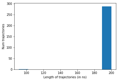
data.dropTraj()
2024-06-12 11:18:13,772 - htmd.metricdata - INFO - Dropped 1 trajectories from 288 resulting in 287
array([145])
Dimensionality reduction#
tica = TICA(data, 20)
dataTica = tica.project(3)
Clustering#
dataTica.cluster(MiniBatchKMeans(n_clusters=200), mergesmall=5)
2024-06-12 11:18:16,315 - htmd.metricdata - INFO - Mergesmall removed 0 clusters. Original ncluster 200, new ncluster 200.
MSM analysis and visualization#
model = Model(dataTica)
model.plotTimescales(lags=list(range(1,100,5)), units="ns")
Estimating Timescales: 100%|██████████████████████████████████████████████████████████████████| 20/20 [00:15<00:00, 1.29it/s]
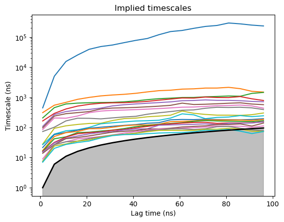
Build Markov Model#
model.markovModel(60, 8, units="ns")
eqDist = model.eqDistribution()
2024-06-12 11:18:33,788 - htmd.model - INFO - 99.7% of the data was used
2024-06-12 11:18:33,803 - htmd.model - INFO - Number of trajectories that visited each macrostate:
2024-06-12 11:18:33,804 - htmd.model - INFO - [ 10   5 287  30  15 111  11  12]
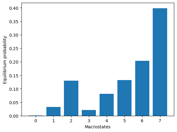
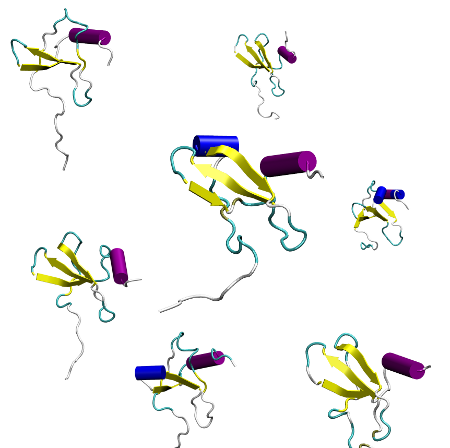
We can now visualize representatives for each of the equilibrium species
model.numsamples=1
model.viewStates(protein=True)
Getting state Molecules: 100%|██████████████████████████████████████████████████████████████████| 8/8 [00:00<00:00, 27.15it/s]
HBox(children=(Checkbox(value=True, description='macro 0'), Checkbox(value=True, description='macro 1'), Check…
NGLWidget()
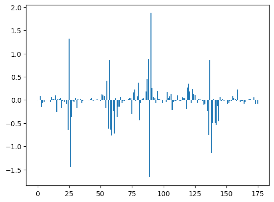
Statistics: What are the major differences between the states X and Y?#
means = getStateStatistic(model, data, range(model.macronum))
plt.figure()
plt.bar(range(len(means[0])), means[-1] - means[-2])
idx = np.where(np.abs(means[-1] - means[-2]) > 0.6)[0]
data.map.iloc[idx]
| type | atomIndexes | description | |
|---|---|---|---|
| 24 | dihedral | [253, 255, 262, 264] | Sine of angle of (SER 16 N A A) (SER 16 CA A A... |
| 25 | dihedral | [253, 255, 262, 264] | Cosine of angle of (SER 16 N A A) (SER 16 CA A... |
| 26 | dihedral | [262, 264, 266, 279] | Sine of angle of (SER 16 C A A) (HSD 17 N A A)... |
| 56 | dihedral | [371, 373, 391, 393] | Sine of angle of (LYS 24 N A A) (LYS 24 CA A A... |
| 57 | dihedral | [371, 373, 391, 393] | Cosine of angle of (LYS 24 N A A) (LYS 24 CA A... |
| 58 | dihedral | [391, 393, 395, 408] | Sine of angle of (LYS 24 C A A) (HSD 25 N A A)... |
| 59 | dihedral | [391, 393, 395, 408] | Cosine of angle of (LYS 24 C A A) (HSD 25 N A ... |
| 61 | dihedral | [393, 395, 408, 410] | Cosine of angle of (HSD 25 N A A) (HSD 25 CA A... |
| 88 | dihedral | [517, 521, 529, 531] | Sine of angle of (PRO 32 N A A) (PRO 32 CA A A... |
| 89 | dihedral | [517, 521, 529, 531] | Cosine of angle of (PRO 32 N A A) (PRO 32 CA A... |
| 90 | dihedral | [529, 531, 533, 543] | Sine of angle of (PRO 32 C A A) (ASN 33 N A A)... |
| 136 | dihedral | [711, 713, 723, 725] | Sine of angle of (ASN 44 N A A) (ASN 44 CA A A... |
| 137 | dihedral | [711, 713, 723, 725] | Cosine of angle of (ASN 44 N A A) (ASN 44 CA A... |
| 138 | dihedral | [723, 725, 727, 737] | Sine of angle of (ASN 44 C A A) (ASN 45 N A A)... |
# we can visualize which residues are different between states
filtered = Molecule('./cxcl12_filtered/filtered.pdb')
filtered.view(sel='protein',style='NewCartoon',hold=True)
filtered.view(sel='resid 16 17 24 25 32 33 44 45',style='Licorice')
NGLWidget()
Mapping back: Which trajectory originated the state X?#
np.where(model.macro_ofmicro == 6)
(array([ 7, 8, 42, 51]),)
_,rel = model.sampleStates(10, 10, statetype='micro')
print(rel)
[array([[ 166, 1371],
       [ 234,  806],
       [ 149, 1108],
       [  80,  666],
       [ 265,  812],
       [  87, 1404],
       [ 243,  370],
       [ 157, 1808],
       [ 204, 1231],
       [ 166, 1656]])]
print(model.data.simlist[232])
simid = 234
parent = None
input = []
trajectory = ['./cxcl12_filtered/9x11/9x11-GERARD_VERYLONG_CXCL12_confAna-0-1-RND0109_9.filtered.xtc']
molfile = ['./cxcl12_filtered/filtered.pdb', './cxcl12_filtered/filtered.psf']
numframes = [None]
Studying a defined reaction coordinate#
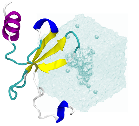
Revising the literature related to CXCL12, we find a paper published by Andrea Bernini et al. (2014), where they describe the opening of a pocket in CXCL12 located between the 2nd and 3rd beta sheet (see figure). To try to capture this phenomenon in our simulations, we will project our trajectories along the 2nd and 3rd beta-sheet distance.
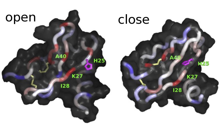
openclose_struc#
Figure taken from Bernini et al., 2014, 1844(3):561-6. DOI:10.1016/j.bbapap.2013.12.012.
The first selection corresponds to beta-sheet 2 carbons alpha, the
second one to beta-sheet 3 CA. We specify metric='contacts' to
create contact maps instead of proper distances. This means: create an
interatom matrix and with 1’s if the distance is below cutoff and 0’s
otherwise.
metr = Metric(fsims)
metr.set(MetricDistance('resid 38 to 42 and noh', 'resid 22 to 28 and noh', periodic=None, metric='contacts'))
data3 = metr.project()
Projecting trajectories:  54%|█████████████████████████████████▍                            | 156/289 [00:21<00:20,  6.51it/s]xtc_read(): XTC file is corrupt
Projecting trajectories: 100%|██████████████████████████████████████████████████████████████| 289/289 [00:40<00:00,  7.22it/s]
2024-06-12 11:21:01,367 - htmd.projections.metric - WARNING - Multiple framesteps [0.0, 0.1] ns were read from the simulations. Taking the statistical mode: 0.1ns. If it looks wrong, you can modify it by manually setting the MetricData.fstep property.
tICA projection#
Dimensionality reduction along the slow process
tica3 = TICA(data3, 20)
dataTica3 = tica3.project(3)
Clustering#
dataTica3.cluster(MiniBatchKMeans(n_clusters=200), mergesmall=5)
2024-06-12 11:22:33,667 - htmd.metricdata - INFO - Mergesmall removed 0 clusters. Original ncluster 200, new ncluster 200.
Plot timescales#
model3 = Model(dataTica3)
model3.plotTimescales(lags=list(range(1,100,5)), units="ns")
Estimating Timescales: 100%|██████████████████████████████████████████████████████████████████| 20/20 [00:01<00:00, 16.92it/s]
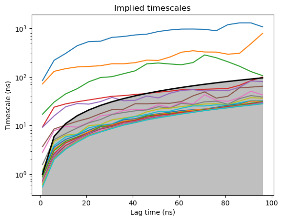
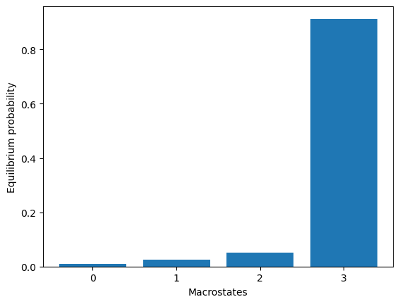
Build a Markov Model#
We want to pick a lagtime where the timescales are converged (timescale is flat). 600 is the lagtime we want to use (600 frames is equivalent to 60ns). 4 is the number of macrostates.
model3.markovModel(60, 4, units="ns")
eqDist = model3.eqDistribution(plot=True)
2024-06-12 11:22:35,487 - htmd.model - INFO - 100.0% of the data was used
2024-06-12 11:22:35,504 - htmd.model - INFO - Number of trajectories that visited each macrostate:
2024-06-12 11:22:35,504 - htmd.model - INFO - [  4   3  19 289]
2024-06-12 11:22:35,505 - htmd.model - INFO - Take care! Macro 1 has been visited only in 3 trajectories (1.0% of total):
2024-06-12 11:22:35,505 - htmd.model - INFO -
simid = 59
parent = None
input = []
trajectory = ['./cxcl12_filtered/3x9/3x9-GERARD_VERYLONG_CXCL12_confAna-0-1-RND1251_9.filtered.xtc']
molfile = ['./cxcl12_filtered/filtered.pdb', './cxcl12_filtered/filtered.psf']
numframes = [None]

2024-06-12 11:22:35,505 - htmd.model - INFO -
simid = 277
parent = None
input = []
trajectory = ['./cxcl12_filtered/10x23/10x23-GERARD_VERYLONG_CXCL12_confAna-0-1-RND9861_9.filtered.xtc']
molfile = ['./cxcl12_filtered/filtered.pdb', './cxcl12_filtered/filtered.psf']
numframes = [None]

2024-06-12 11:22:35,506 - htmd.model - INFO -
simid = 280
parent = None
input = []
trajectory = ['./cxcl12_filtered/10x27/10x27-GERARD_VERYLONG_CXCL12_confAna-0-1-RND0101_9.filtered.xtc']
molfile = ['./cxcl12_filtered/filtered.pdb', './cxcl12_filtered/filtered.psf']
numframes = [None]
Visualize states#
model3.viewStates(protein=True, numsamples=1)
Getting state Molecules: 100%|██████████████████████████████████████████████████████████████████| 4/4 [00:00<00:00, 32.17it/s]
HBox(children=(Checkbox(value=True, description='macro 0'), Checkbox(value=True, description='macro 1'), Check…
NGLWidget()
Analyse Open Conformation#
Did you see any macrostate where the pocket is open? What is the equilibrium population probability? Let’s try to find the trajectory that produced the state…
# Map back the trajectory/ies that originated the macro. Substitute 1 for the macro that showed the pocket opening.
# This function is giving you the microclusters that are inside a given macrocluster
np.where(model3.macro_ofmicro ==1)
(array([ 17, 23, 59, 114, 148]),)
# substitute 48 for the micro number from the previous step
# This function gives you trajectory-frame pairs that visited a given micro
_, rel = model3.sampleStates(48, 5, statetype='micro')
print(rel)
[array([[  35, 1927],
       [ 180, 1529],
       [ 283,  255],
       [  34, 1400],
       [  67, 1430]])]
print(model3.data.simlist[277])
simid = 277
parent = None
input = []
trajectory = ['./cxcl12_filtered/10x23/10x23-GERARD_VERYLONG_CXCL12_confAna-0-1-RND9861_9.filtered.xtc']
molfile = ['./cxcl12_filtered/filtered.pdb', './cxcl12_filtered/filtered.psf']
numframes = [None]
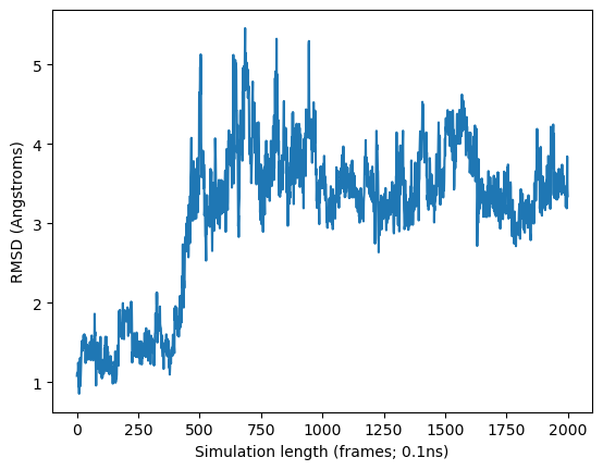
Calculate RMSD of the site of interest for a selected trajectory#
simus = simlist(glob('./cxcl12_filtered/10x23/'), './cxcl12_filtered/')
Creating simlist: 100%|████████████████████████████████████████████████████████████████████████| 1/1 [00:00<00:00, 173.87it/s]
refmol = Molecule('./cxcl12_filtered/filtered.pdb')
metr = Metric(simus)
metr.set(MetricRmsd(refmol, 'resid 38 to 42 or resid 22 to 28 and noh'))
rmsd = metr.project()
Projecting trajectories: 100%|██████████████████████████████████████████████████████████████████| 1/1 [00:00<00:00,  2.58it/s]
2024-06-12 11:22:50,859 - htmd.projections.metric - INFO - Frame step 0.1ns was read from the trajectories. If it looks wrong, redefine it by manually setting the MetricData.fstep property.
Do you see the pocket opening at 50ns?#
plt.plot(rmsd.dat[0])
plt.xlabel('Simulation length (frames; 0.1ns)', fontsize=10)
plt.ylabel('RMSD (Angstroms)', fontsize=10)
plt.show()
Visualize the trajectory from your browser#
refmol.read('./cxcl12_filtered/10x23/10x23-GERARD_VERYLONG_CXCL12_confAna-0-1-RND9861_9.filtered.xtc')
refmol.align('protein')
refmol.view()
NGLWidget(max_frame=1999)
This concludes the conformational analysis tutorial