How to read off and interpret an implied-timescales plot#

Goal#

Pick a Markov lag time + a number of macrostates from plotTimescales() output, and recognise common pathologies (insufficient lag, undersampling, fake macrostates) before they bake into the final model.

Minimal example#

from htmd.model import Model

model = Model(dataBoot)
model.plotTimescales(maxlag=40, units="ns")

The plot shows several curves - one per slow process - of implied timescale vs Markov lag time. The X axis is the lag time you’d pass to model.markovModel(lag, ...); the Y axis is the timescale that lag-time would imply.

How to read it#

A correct ITS plot has three features:

Plateau region: each curve flattens out (vs the diagonal) as lag increases. The lag time at which the curves first plateau is your Markov lag.
Gap pattern: a clear vertical gap between the top k curves and the bottom-of-the-plot continuum means there are k slow processes - the system has k + 1 macrostates.
No gross monotonic drift: timescales should bounce around their plateau value with small statistical noise, not keep climbing linearly with lag.

Pick the shortest lag at which the top curves have plateaued - that maximises kinetic resolution without breaking Markovianity. Pick macronum = (number of distinct slow timescales) + 1.

Common patterns#

Healthy ITS plot#

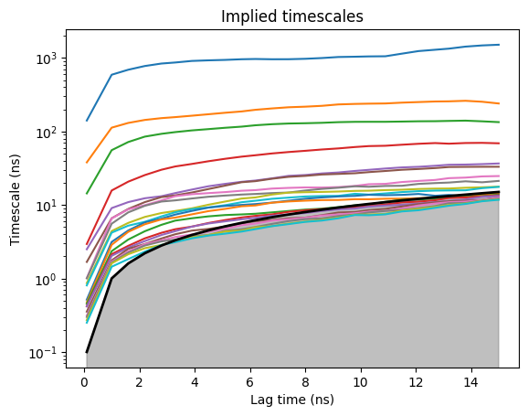
Implied timescales plot for the trypsin-benzamidine binding system

This is the ITS plot from the trypsin-benzamidine binding tutorial. Reading it:

Three slow processes stand clearly above the continuum: the slowest (blue, ~1500 ns), the second (orange, ~200 ns), and the third (green, ~130 ns).
Plateau region: every curve climbs sharply from lag ≈ 0 then flattens out by lag ≈ 4 ns. Pick the shortest plateau lag - lag ≈ 4 ns here.
Grey shaded region below: the line where timescale = lag. Curves inside this region are kinetically meaningless (you can’t resolve a process faster than the lag you sampled it with).

With three slow processes clearly separated from the dense lower continuum, set markovModel(lag=4, macronum=4, units="ns") (3 slow processes → 4 metastable basins).

Drifting / non-plateauing curves#

If every curve keeps climbing linearly with lag, the underlying data is non-Markovian at this resolution - your microstate decomposition is too coarse, or your projection misses a slow degree of freedom. Re-cluster with more microstates, or change the features in your projection so they can capture the slowest degrees of freedom of the system.

Pathological gap#

A “gap” that disappears at higher lag, or that’s noisy across bootstraps, isn’t a real macrostate boundary. Bootstrap and look at the variance (see how-to).

Inverted timescales#

Timescales that decrease with lag almost always mean an over-clustering bug or a numerical artefact. Re-cluster with fewer microstates and re-fit.

Common variations#

Limit to the N slowest processes#

model.plotTimescales(maxlag=40, units="ns", nits=5)

By default plotTimescales() plots up to min(K-1, 20) slowest timescales (where K is the number of microstates). Pass nits=5 to keep only the 5 slowest curves - useful when the continuum below them is noisy.

Bootstrapped ITS#

See How to bootstrap a model for error bars - re-run the ITS plot on each bootstrap and overlay; mean ± stdev across bootstraps tells you whether the plateau is sample-stable.

Compare lag times by direct call#

for lag in [5, 10, 20, 40]:
    model.markovModel(lag, macronum=4, units="ns")
    slowest_ns = model.msm.timescales()[0] * model.data.fstep
    print(f"lag={lag} ns -> slowest = {slowest_ns:.1f} ns")

model.msm.timescales() (deeptime API) returns the implied timescales in the same units as model.lag - htmd stores the lag in frames after the unit conversion from markovModel(..., units=...), so the values come back in frames. Multiply by model.data.fstep to get ns. Useful for quickly confirming the plateau choice without rerunning the full plot.

Gotchas#

Pick the shortest plateau-lag, not the highest one. Higher lag throws away both samples (fewer transition counts available at long lags) and kinetic resolution, for no Markovianity gain.
A clean plateau on a single un-bootstrapped fit can be deceptive. Always bootstrap and look at variance across replicates before settling on a lag.
“Number of slow processes” reads off as the number of curves visibly above the continuum. If your gap is fuzzy, your data probably doesn’t support that many macrostates - reduce macronum.
The ITS plot’s axis labels are always "Lag time (ns)" / "Timescale (ns)" - hardcoded regardless of the units= argument you pass. Only data.fstep controls the absolute numeric scale; if fstep is wrong (or unset) the labels still claim “ns” but the numbers are in whatever unit fstep actually represents.