Ligand binding MSM: trypsin + benzamidine

You will learn: how to take unbiased binding trajectories of a small drug-like ligand and a protein receptor and build a Markov-state model that gives you the bound macrostate, the binding pathways, the binding affinity (K_d), and on / off rates.

Prerequisites:

• HTMD installed.

• wget available on $PATH.

• ~5 GB of disk for the trajectory download.

The system

Trypsin is a serine protease; benzamidine is a small competitive inhibitor that docks into the S1 specificity pocket. The dataset contains short unbiased trajectories started from many random ligand poses around the protein - some find the binding pocket, most don’t. Aggregate sampling is ≈ 17 µs across 852 trajectories.

The point of this analysis is to reconstruct the binding free-energy surface and rates without ever steering the ligand - just by counting transitions between metastable states discovered by clustering the trajectories.

The flow

Same MSM pipeline as the villin folding tutorial - the only thing that changes is the projection: for a binding problem the slow coordinate is the protein-ligand distance pattern, not the protein’s own contact map.

1. Download + simlist.

2. Project with MetricDistance between protein Cα atoms and ligand heavy atoms.

3. TICA to find the slow binding modes.

4. Cluster, build MSM, lump into macrostates.

5. Read out the FES, MFPTs, k_on / k_off, and K_d.

Setup

import os
from glob import glob
from pathlib import Path
from htmd.ui import (
    simlist, simmerge,
    Metric, MetricDistance,
    TICA, Model, Kinetics,
)
from sklearn.cluster import MiniBatchKMeans

Please cite HTMD: Doerr et al.(2016)JCTC,12,1845. https://dx.doi.org/10.1021/acs.jctc.6b00049
HTMD Documentation at: https://software.acellera.com/htmd/

You are on the latest HTMD version (2.8.5.dev17+gf26491d44.d20260602).

2026-06-02 18:40:37,204 - rdkit - INFO - Enabling RDKit 2026.03.2 jupyter extensions

Step 1 - Build the simlist

The trajectory bundle ships on Figshare (HTMD tutorial data, DOI 10.6084/m9.figshare.32541291) as ligand_binding_datasets.zip (~3 GB).

The dataset is split into several “epochs” (adaptive-sampling rounds). simlist() builds one per-epoch list (duplicate folder basenames within a single call would raise), and simmerge() stitches them into a combined list and renumbers the per-sim simid indices to be sequential across the merged whole:

DATASETS = Path(os.environ["HTMD_TUTORIAL_DATASETS"]) / "ligand_binding_datasets"
topology = str(DATASETS / "1" / "filtered")  # any epoch works - all share the same topology
sims = []
for epoch in sorted(DATASETS.glob("*/")):
    trajs = glob(os.path.join(epoch, "filtered", "*", ""))
    sims = simmerge(sims, simlist(trajs, topology))
len(sims)

852

Step 2 - Project: protein-ligand contacts

For binding, the relevant coordinate is “which protein residue is the ligand currently in contact with”. MetricDistance computes the distance matrix between two atom selections; with metric="contacts" you get a binary contact map per frame between every protein Cα and every ligand heavy atom (1 if the distance is below the threshold, 0 otherwise - default threshold=8 Å).

metr = Metric(sims)
metr.set(MetricDistance(
    "protein and name CA",
    "resname MOL and noh",
    periodic="selections",
    metric="contacts",
))
data = metr.project()
data.fstep = 0.1

htmd.projections.metric - INFO - Frame step 0.001ns was read from the trajectories. If it looks wrong, redefine it by manually setting the MetricData.fstep property.

data.plotTrajSizes()
data.dropTraj()

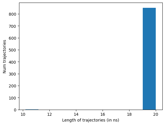
htmd.metricdata - INFO - Dropped 2 trajectories from 852 resulting in 850

array([496, 562])

periodic="selections" makes the distance calculation use minimum-image distances between the two atom selections, so a ligand that has wrapped through PBC gets compared to the closest protein image - the original coordinates aren’t modified, only the distances are computed correctly across the box.

Step 3 - TICA

tica = TICA(data, 2, units="ns")
dataTica = tica.project(3)

Step 4 - Cluster + MSM

dataBoot = dataTica.bootstrap(0.8)
dataBoot.cluster(MiniBatchKMeans(n_clusters=1000))

model = Model(dataBoot)
model.plotTimescales(maxlag=15, units="ns")

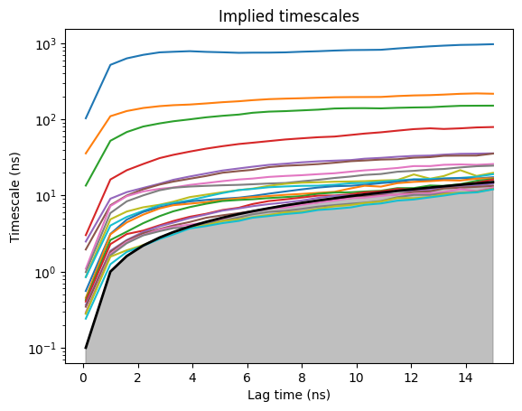
The slow timescale for binding is much shorter than folding (ligand diffusion happens on the ns-100ns scale, not µs). Read the lag off the ITS plot - usually around 5 ns for this system.

model.markovModel(5, 5, units="ns")

htmd.model - INFO - 100.0% of the data was used
htmd.model - INFO - Number of trajectories that visited each macrostate:
htmd.model - INFO - [153 105 376 127 220]

Five macrostates: bound + a few “encountered but not docked” intermediates + the bulk solution.

Step 5 - Free-energy surface

model.plotFES(0, 1, temperature=298)

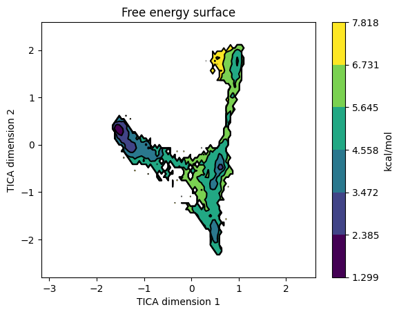
model.plotFES(0, 1, temperature=298, states=True)

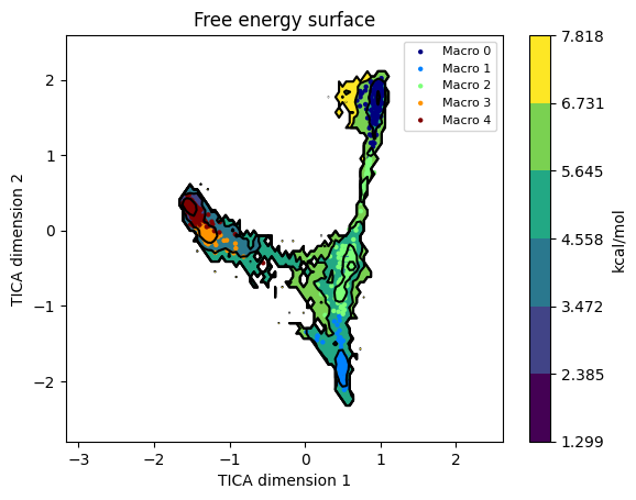
The bound state usually appears as a deep basin in one corner of TIC1 / TIC2; the bulk-solution state spreads across most of the projected area; the intermediates are shallow basins between them.

To overlay representative protein + ligand snapshots from each macrostate, run model.viewStates(ligand="resname MOL and noh") from an interactive session - it launches VMD. (Omitted here because it needs a display.)

Step 6 - Kinetics + K_d

kin = Kinetics(model, temperature=298, concentration=0.0037)

htmd.kinetics - INFO - Detecting source state...
htmd.kinetics - INFO - Guessing the source state as the state with minimum contacts.
htmd.kinetics - INFO - Source macro = 2
htmd.kinetics - INFO - Detecting sink state...
htmd.kinetics - INFO - Sink macro = 4

concentration=0.0037 mol/L is the effective bulk ligand concentration in this simulation box (one ligand in the periodic box of this volume). Kinetics uses it to convert the simulated rates into experimental units - k_on (M⁻¹ s⁻¹), k_off (s⁻¹), and K_d = k_off / k_on.

r = kin.getRates()
print(r)

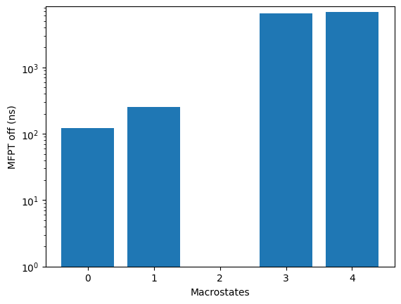
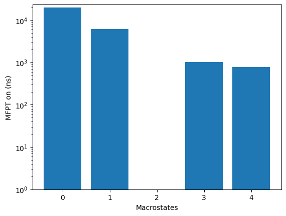
mfpton = 7.88E+02 (ns)
mfptoff = 6.80E+03 (ns)
kon = 3.43E+08 (1/M 1/s)
koff = 1.47E+05 (1/s)
koff/kon = 4.29E-04 (M)
kdeq = 3.58E-04 (M)
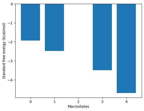
g0eq = -4.70 (kcal/M)

htmd.kinetics - INFO - Calculating rates between source: [np.int64(2)] and sink: [np.int64(4)] states.
htmd.kinetics - INFO - Concentration correction of -3.32 kcal/mol.

getRates() returns a single Rates object for the auto-detected source → sink pair (bulk → bound here). It carries the MFPT, rate, and k_on / k_off / K_d. Match against the experimental K_d to validate the model. Use kin.plotRates() (below) for an all-pairs visualisation, or call getRates(source=..., sink=...) explicitly for other pairings.

kin.plotRates()

kin.plotFluxPathways()

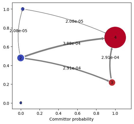
Path flux		%path	%of total	path
0.00038753881932143707	55.4%	55.4%		[2 4]
0.00029093136484922627	41.6%	97.0%		[2 3 4]
2.0777315285460142e-05	3.0%	100.0%		[2 1 4]

The flux pathways show which intermediates the ligand visits on the way from solution to the bound pocket - useful for understanding the binding mechanism (e.g. is there a kinetic trap on the surface? Does the ligand approach from a specific direction?).

Parameters that matter

Knob	Effect
MetricDistance(sel1, sel2, ... metric="contacts")	Coarse but the right default for binding - thresholding collapses the huge unbound bulk region into a single “no contacts” state. metric="distances" would spread that bulk across thousands of useless microstates and overwhelm the bound-state resolution.
threshold on MetricDistance	Default 8 Å. Lower (e.g. 5 Å) tightens what counts as “in contact” and emphasises tighter poses; higher dilates the bound basin.
concentration on Kinetics	Critical for kon and Kd. Compute it as (nligands / nwaters) · 55.4 mol/L - the water count tracks the real bulk volume more accurately than the box volume, which over-counts because it includes the protein’s excluded volume.
periodic="selections" on the projection	Essential when the ligand wraps through the box during the trajectory. Skipping it produces nonsense contacts at PBC crossings.
model.markovModel(lag, macronum) macronum	More macrostates → more pathway resolution but harder to interpret. 4-6 is typical for binding.

Gotchas

• The bulk state is huge and unstructured. With metric="contacts" the unbound bulk collapses to essentially a single microstate (all-zero contact vector), which is exactly what you want for binding analysis. Don’t over-interpret intermediate basins that have very small populations - they may be undersampled.

• Bound-state validation. Before trusting K_d, open viewStates(ligand=...) and confirm the bound macrostate actually puts the ligand in the experimental pocket. If it’s binding to the wrong site, your model is sampling a metastable mis-pose.

• Symmetric ligands. Benzamidine is roughly C₂v-symmetric; for ligands without that symmetry, atom-pair distances can flip when the ligand rotates 180°. Either symmetrise the contact features manually or accept that the model will distinguish the two flipped orientations as separate states.

See also

• MSM workflow explanation - what’s happening under the hood.

• Protein folding MSM - same pipeline, different projection.

• Adaptive sampling - how the binding trajectory set was generated (random starting poses + adaptive sampling targeting under-explored regions).